


Microsoft Excel | Page Six | Profit/Loss and VAT
Walk throughs focus on formulae (pl) but you might also endeavour to apply formatting (illustrated) where appropriate.
Page: 1 of 6 | 2 of 6 | 3 of 6 | 4 of 6 | 5 of 6 | 6 of 6
Profit/Loss and VAT
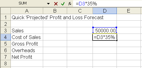
Applying formulae to achieve a 'projected' profit and loss forecast
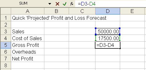
The following forecast shows a fixed sales figure of £50,000.00 at cell: D3. Cell D4 calculates 35% of sales (D3) assuming a mark-up/gross profit of 65% – this will perhaps be numerical data (not necessarily a formula calling data from another cell).
The gross profit at D5 is actual sales (D3) less the cost the sales (D4).
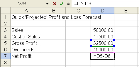
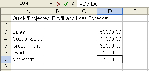
D6 assumes a fixed figure of £15,000.00. The net profit at cell D7 is gross profit (D5) less overheads at cell D6.
Applying formulae for simple profit and loss
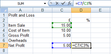
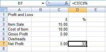
An item costing £10.00 sold for £15.00 represents a mark-up of 50% – the profit however is not 50%. Profit and loss must take account of the item cost, and consequently the percentage return in the following example is 33% (of £15.00), i.e. the item profit is 33% taking into account the purchase price.
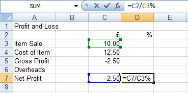
An item costing £12.50 sold for £10.00 represents a mark-down of 25%. The profit/loss in the following example is -25% (of £10.00), i.e. the item loss is 25% taking into account the purchase price.

A more complex profit and loss layout calculating margins
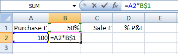
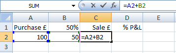
If goods purchased cost £100.00 and the margin is 50% giving us a £50.00 increase, the profit/loss is 33% of the total (return). See below:
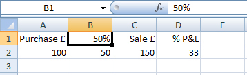
To work out the profit/loss, first of all apply your % increase to your column heading, see B1 (Not necessarily a fixed percentage… 50% in this example. Format the cell to percentage, 0 decimal places – include the other column headings as shown.
In cell B2 beneath your % heading, enter: =A2*B$1
The purchase price at A2 is multiplied by the percentage entered at B1 – the reference (at B2) to row 1 at cell B1 fixed with an Absolute reference ($).
The sale price is the purchase price at A2 plus the margin/mark-up at B2 (=A2+B2). The profit/loss is the resulting margin % at B2 divided by sale price at C2 (=B2/C2%).
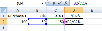
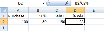
Note that changing the purchase price in cell A2 will automatically increase the margin in B2 (Resulting from the formula in that cell) as well as the sale price in C2, but the % profit and loss (D2) will remain the same.
Illustrations above are based on a margin set at 50%. To see a change in the total % profit and loss, change the % increase at B1.
Applying formulae to facilitate a 'random' profit and loss entry
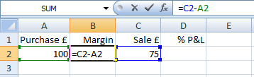
First of all apply a formula to work out the margin (mark-up/mark-down) in price, e.g. = sale price (Cell reference, not amount) less purchase price (=C2-A2).
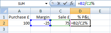
The sale price in this example is whatever you enter in C2. The % profit/loss is the resulting margin in B2 divided by the sale price (=B2/C2%).
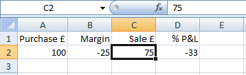
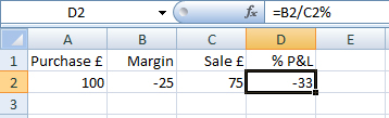
Note above that while the sale price in the illustration is clearly 25% less than the cost price, the profit/poss is the margin as a percentage of the sale price (the margin as a percentage of the total re-sale price, e.g. purchase price plus/minus the margin (33%)).
An accountant will perhaps simply record a loss as a NIL return. The above guidelines may require some clarification, if you can help please complete the online form.
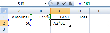
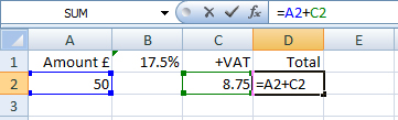
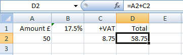
Applying formulae to work out what value added tax to add
Here we multiply the cell reference (Amount (A2)) by the VAT (change to current rate, e.g. 20%) fixed in one cell (B1), then add together with the amount (A2) to give a total. Remember to fix ($) reference to cell B1 if replicating down for example (=A2*B$1).
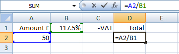
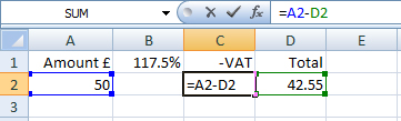
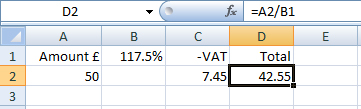
Applying formulae to work out what value added tax is included
To work out how much VAT has been included in a total, firstly divide the cell reference (Amount (A2)) by 100+VAT rate (e.g. 120% From January 4, 2011) fixed in one cell (B1), to formulate the total (D2), before subtracting from the amount at A2 (See: C2). Remember to fix ($) reference to cell B1 if replicating down.
For example: =A2/B$1 (See: Absolute reference).
The power of Excel
For the advanced, or those who simply might like to look at more complex formulae, download the following Excel File (Sheets x2) to analyse possible or potential complexity in numeric modules – The file may take awhile to open (Microsoft Office Excel Required).
The spreadsheet was structured for a client who wanted to monitor progress of a World Championship Dance Competition. Judged by three independent adjudicators, the worksheet needed a score-table (Sheet 2).
![]() Commissioned some years ago, I'm not able to go into detail – you might nonetheless like to look at formulae in the RANK, and SCORE columns on Sheet 1 (Feis), and then the LOOKUP AND COUNTIF columns on Sheet 2 (Lookup).
Commissioned some years ago, I'm not able to go into detail – you might nonetheless like to look at formulae in the RANK, and SCORE columns on Sheet 1 (Feis), and then the LOOKUP AND COUNTIF columns on Sheet 2 (Lookup).
Best wishes
PCWorkspace
