Microsoft Excel | Page One | Cell Reference
The following Excel '97 – 2010 tutorial is structured to assist together with your Microsoft Office Excel application, assumes some proficiency in text processing. Please note that these pages focus on formulae (pl) but you might also endeavour to apply formatting (illustrated) where appropriate.
Page: 1 of 6 | 2 of 6 | 3 of 6 | 4 of 6 | 5 of 6 | 6 of 6
Open your Excel application. It's important first of all to emphasise that cells within a worksheet are identified by a sequential reference, and to further illustrate how we arrive at this reference.
Note that in the following diagram the letters (A-Z (Grey segments across the top)) apply to the columns down, and that the numbers (1… 65,536 (Illustrated down the left side of your worksheet)) apply to the rows across.
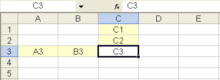
Cell reference is essentially the cell label, the tag allocated to each cell within a worksheet. Important because it is the cell reference (pointing to the numerical data) that is referred to in the make-up of formulae.
For example: =A3+B3
Where cell A3 contains numerical data, cell B3 contains numerical data, and the formula: =A3+B3 has been entered into cell C3, the result would be the sum total of both of the cells (A3 + B3) containing the data (See below).
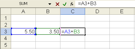
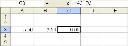
Note that the result is displayed in the formula cell, and that the formula can also be seen in the formula bar above the worksheet.

Once again it is important to note that the cell reference is used in the make-up of formulae, not the numerical data. Entering some data and illustrating is perhaps the simplest way to explain why.
Open a spreadsheet, enter some data and a formula by clicking directly into the formula bar or the cell itself. The results will show in the formula/total cell when the data is confirmed (enter key returned or another cell selected).
Observe the result, amend the numerical data in one of the cells, e.g. edit cell A3, updating from 5.50 to 8.50, and note the change in the formula/total cell at C3.
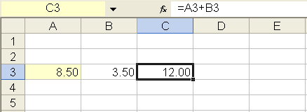
The formula (above (See: formula bar)) refers to the cell(s) regardless of content. The total is automatically updated when change to numerical data is applied. When a cell is selected, the reference to the cell can be seen to the left of the formula bar.

For later
To jump to a particular cell, in an extensive spreadsheet for example, enter the cell reference in the section above your worksheet, to the left of the formula bar.
You can also allocate your own label to a cell, e.g. 'Home' for cell A1. To do this, select cell A1 and enter 'Home' in the section to the left of the formulae bar. Click on the down-arrow to choose a previously personalised cell location from the drop-down menu.
Before you continue
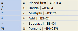
Basic characters (signs (keyboard symbols)) used in the make-up of formulae:

Calculating more than two cells
In the above illustration, I added the contents of two cells together keeping it simple. Now lets add a string of cells together.
It might be an idea to keep numerical data simple at first, conceivably allowing to mentally total figures, perhaps helping to build confidence.
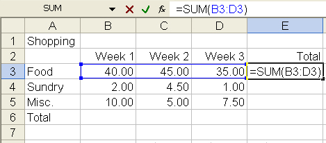
Enter some shopping data. Select an appropriate cell where a total is to be calculated, and enter the =SUM() formula, including the range of cells within the parenthesis. The range is the first and last data cell separated by a colon.
For example: =SUM(B3:D3)
In other words, B3 through D3, the sum total of these cells, any number of cells adjacent in a row or column. In the following diagrams, I firstly add together all items in row 3, the three cells B3, C3, and D3 (Food), then I calculate column B (Week 1).
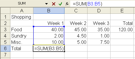
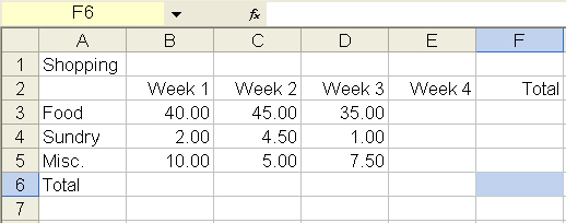
Total the Sundry and Miscellaneous rows and the remaining columns. Only weeks one to three are included – you might like to adapt the worksheet to include week four.
A grand total can be achieved by either totalling the 'Total' column above, or the 'Total' row to the left. If the numerical data has been entered correctly, both will give the same answer – a simple means perhaps to cross-check your data in a large worksheet.
How to achieve an average
=AVERAGE()
Place the range between the parenthesis – at cell reference F3: =AVERAGE(B3:E3) allowing for week 4. Modify your formula to return a monthly average.
=AVERAGE()*52/12
Place the range between the parenthesis, multiplying by 52 weeks and dividing by 12 months – e.g. at cell reference F3: =AVERAGE(B3:E3)*52/12 allowing for week 4.


